Guide

A cookbook of common tasks. Every example assumes using EntroPlots and reuses the DNA PFM below (a 4 × N matrix whose columns sum to 1):

using EntroPlots

pfm = [0.02  1.0  0.98  0.0   0.0   0.0   0.98  0.0   0.18  1.0
       0.98  0.0  0.02  0.19  0.0   0.96  0.01  0.89  0.03  0.0
       0.0   0.0  0.0   0.77  0.01  0.0   0.0   0.0   0.56  0.0
       0.0   0.0  0.0   0.04  0.99  0.04  0.01  0.11  0.23  0.0]

logoplot(pfm)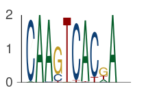

Custom background frequencies

By default each symbol is scored against a uniform background. Pass your own background (order A, C, G, T) to score information content against it instead:

logoplot(pfm, [0.3, 0.2, 0.2, 0.3])

Minimal styling (no margins, no axes)

using Plots  # for `Plots.mm`
logoplot(pfm; _margin_=0Plots.mm, tight=true, yaxis=false, xaxis=false)

Highlight regions of interest

Pass a vector of position ranges to shade selected columns:

logoplot_with_highlight(pfm, [4:8])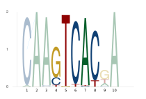

Tight variant (no surrounding margin):

using Plots
logoplot_with_highlight(pfm, [4:8]; _margin_=0Plots.mm, tight=true)

Protein motifs (20 amino acids)

Protein PFMs are 20 × N. Use reduce_entropy! to sharpen each column toward its dominant residue — helpful for noisy matrices — then set protein=true:

matrix = rand(20, 25)
pfm_protein = matrix ./ sum(matrix, dims=1)
reduce_entropy!(pfm_protein)  # sharpen toward dominant residue per column

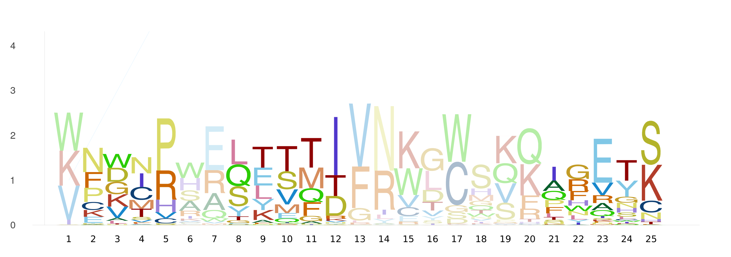
logoplot(pfm_protein; protein=true)
logoplot_with_highlight(pfm_protein, [2:5, 8:12, 21:25]; protein=true)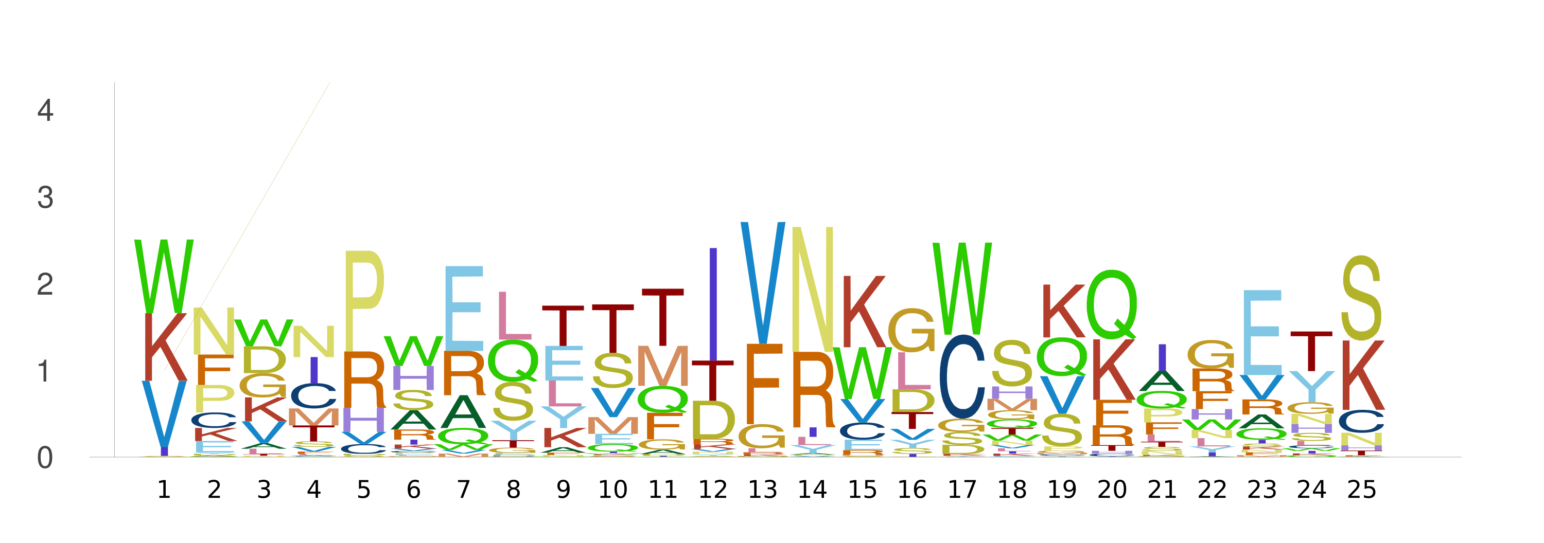

RNA motifs

logoplot(pfm; rna=true)  # uses A, C, G, U

Saving to file

The output format is inferred from the file extension (PNG, SVG, …):

save_logoplot(pfm, "logo.png")                          # default uniform background
save_logoplot(pfm, [0.3, 0.2, 0.2, 0.3], "logo.png")    # custom background
save_logoplot(pfm_protein, "protein.png"; protein=true)
save_logoplot(pfm, "highlighted.png"; highlighted_regions=[4:8])

Gapped logos with strike-through connectors

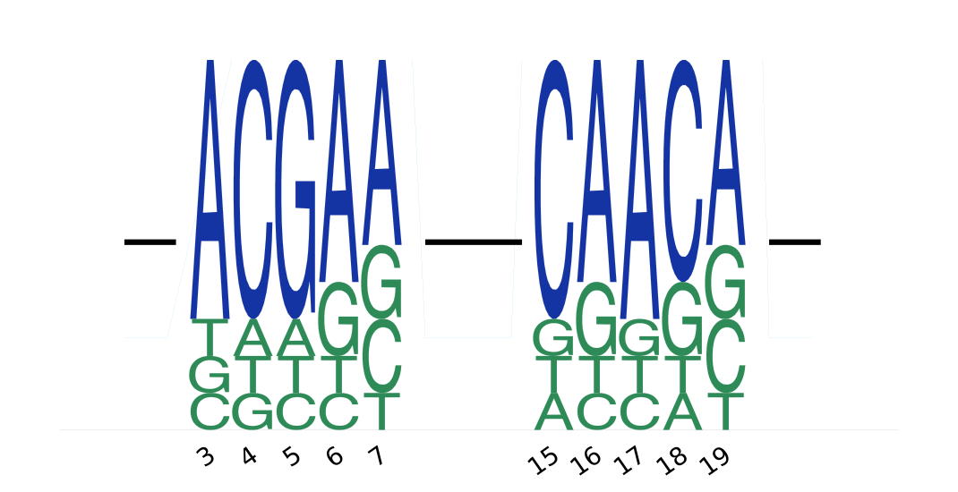
To lay several logo fragments along a single track — with the gaps between them drawn as a strike-through line — use logoplot_with_rect_gaps (or save_logo_with_rect_gaps to write straight to a file).

Unlike logoplot, this takes integer count matrices (rows = A, C, G, T; not normalized PFMs), a starting position for each fragment, and the total_length of the track. The empty regions between fragments become the strike-through connectors.

Optionally pass a one-hot reference_pfms (a BitMatrix per fragment) to color each letter by whether it matches or differs from the reference — handy for showing mutations against a wild-type sequence.

using EntroPlots

# Integer COUNT matrices (rows = A, C, G, T) — NOT normalized PFMs.
cm1 = [70 10 10 60 50
       10 70 10 10 20
       10 10 70 20 20
       10 10 10 10 10]

cm2 = [10 60 70 10 50
       70 10 10 60 20
       10 20 10 20 20
       10 10 10 10 10]

# One-hot reference per fragment (BitMatrix): match vs. mismatch coloring.
ref1 = BitMatrix([1 0 0 1 1
                  0 1 0 0 0
                  0 0 1 0 0
                  0 0 0 0 0])
ref2 = BitMatrix([0 1 1 0 1
                  1 0 0 1 0
                  0 0 0 0 0
                  0 0 0 0 0])

count_matrices   = [cm1, cm2]
starting_indices = [3, 15]   # start position of each fragment on the track
total_length     = 22        # gaps between fragments -> strike-through line

save_logo_with_rect_gaps(
    count_matrices, starting_indices, total_length,
    "logo_rect_gaps.png";
    reference_pfms     = [ref1, ref2],
    dpi                = 100,
    xrotation          = 35,
    uniform_color      = true,
    ref_match_color    = "#1434A4",   # blue: matches reference
    ref_mismatch_color = "#2E8B57",   # green: differs from reference
)

Set filter_by_reference=true to first drop columns that exactly match the reference (via apply_count_filter), keeping only the positions that vary. To draw the plot without saving, call logoplot_with_rect_gaps with the same arguments (minus the file path).

Amino-acid (protein) variant

The same works for protein motifs — pass protein=true and supply 20-row count matrices and references (rows in the order A C D E F G H I K L M N P Q R S T V W Y):

using EntroPlots

# 20 amino acids, in the row order EntroPlots expects.
const AA = ["A","C","D","E","F","G","H","I","K","L",
            "M","N","P","Q","R","S","T","V","W","Y"]
row(c) = findfirst(==(c), AA)

# 20 x ncols COUNT matrix: small background, a tall dominant residue per column,
# plus a shorter secondary residue for a realistic stack.
function counts(dominant, secondary; base=1, hi=90, mid=30)
    M = fill(base, 20, length(dominant))
    for j in eachindex(dominant)
        M[row(dominant[j]),  j] += hi
        M[row(secondary[j]), j] += mid
    end
    return M
end

# One-hot reference (BitMatrix): the wild-type residue per column.
onehot(seq) = BitMatrix([AA[i] == seq[j] for i in eachindex(AA), j in eachindex(seq)])

# Fragment 1: dominant motif L K E F ; reference (wild-type) L K D F
cm1  = counts(["L","K","E","F"], ["I","R","D","Y"])
ref1 = onehot(["L","K","D","F"])   # column 3 differs (E vs D) -> mismatch color

# Fragment 2: dominant motif R S T Y ; reference R A T Y
cm2  = counts(["R","S","T","Y"], ["K","T","V","F"])
ref2 = onehot(["R","A","T","Y"])   # column 2 differs (S vs A) -> mismatch color

save_logo_with_rect_gaps(
    [cm1, cm2], [3, 12], 17,          # starts at 3 and 12, total track length 17
    "logo_rect_gaps_protein.png";
    protein            = true,
    reference_pfms     = [ref1, ref2],
    dpi                = 100,
    xrotation          = 35,
    uniform_color      = true,
    ref_match_color    = "#1434A4",   # blue: matches reference
    ref_mismatch_color = "#2E8B57",   # green: differs from reference
)

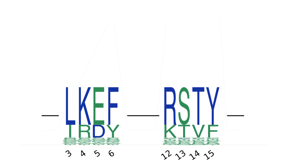
Here LKEF and RSTY are the dominant motifs; the reference-mismatch columns (E in fragment 1, S in fragment 2) are drawn in green, everything matching the wild-type in blue.

Common keyword arguments

Most plotting functions accept the following keywords:

See the API Reference for the full signatures and per-function options.